
Tracking

On December 17th 2010 I started using Google Latitude on my phone. It didn’t really take off as a location sharing application but I thought it was pretty cool that I’d have access to all this interesting information.
All the data is exportable and you can plot it on a map, however I was looking to create a nice looking map rather than the static lines between points that are shown in Google Earth if you import the exported KML file.
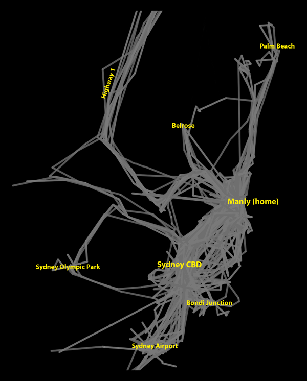
So I followed this guide at flowing data which uses great circles to plot lines between points on a map. The results are really impressive, here’s my general travel in and around Sydney. I’ve removed the backing map and just added indicators of some of the locations, as I think the lines alone look nice, the slightly different colours are based on if the travel was made from East to West or West to East. You can see the route you have to take to get to Highway 1 from Manly (there’s a national park in the way) –

Taking it to the next level I’ve plotted my travels across the globe since December 17th 2010 (click it for the larger version) –

If you’ve been tracking yourself on Latitude then export the KML, covert it to a CSV file with just the lat/lon results. Import them into R and use this code to plot them on a map (follow the flowing data tutorial first) –
movements <- read.csv("http://yourserver.com/yourLatLon.csv",header=TRUE, col.names=c("lat","lon"))
xlim<-c(-10,180)
ylim<-c(-50,70)
map("world",col="#efefef",fill=TRUE,bg="white",lwd=0.02,xlim=xlim,ylim=ylim)
for(j in 2:(length(movements$lat)-1)) {
 lat_ca<- movements$lon[j]
 lon_ca<- movements$lat[j]
 lat_me<- movements$lon[j-1]
 lon_me<- movements$lat[j-1]
 inter <- gcIntermediate(c(lon_ca, lat_ca), c(lon_me, lat_me), n=50, addStartEnd=TRUE)

 if ( lat_ca < lat_me ) coll=rgb(0.251,0.47,0.47,alpha=0.8) else coll=rgb(0.251,0.129,0.47,alpha=0.8)

 lines(inter,col=coll,lwd=2)
}